Introduction

Sorting data means arranging it in a certain order, often in an array-like data structure. You can use various ordering criteria, common ones being sorting numbers from least to greatest or vice-versa, or sorting strings lexicographically. You can even define your own criteria, and we'll go into practical ways of doing that by the end of this article.

If you're interested in how sorting works, we'll cover various algorithms, from inefficient but intuitive solutions, to efficient algorithms which are actually implemented in Java and other languages.

There are various sorting algorithms, and they're not all equally efficient. We'll be analyzing their time complexity in order to compare them and see which ones perform the best.

The list of algorithms you'll learn here is by no means exhaustive, but we have compiled some of the most common and most efficient ones to help you get started,

Note: This article will not be dealing with concurrent sorting, since it's meant for beginners.

Bubble Sort

Explanation

Bubble sort works by swapping adjacent elements if they're not in the desired order. This process repeats from the beginning of the array until all elements are in order.

We know that all elements are in order when we manage to do the whole iteration without swapping at all - then all elements we compared were in the desired order with their adjacent elements, and by extension, the whole array.

Here are the steps for sorting an array of numbers from least to greatest:

• 4 2 1 5 3: The first two elements are in the wrong order, so we swap them.

• 2 4 1 5 3: The second two elements are in the wrong order too, so we swap.

• 2 1 4 5 3: These two are in the right order, 4 < 5, so we leave them alone.

• 2 1 4 5 3: Another swap.

• 2 1 4 3 5: Here's the resulting array after one iteration.

Because at least one swap occurred during the first pass (there were actually three), we need to go through the whole array again and repeat the same process.

By repeating this process, until no more swaps are made, we'll have a sorted array.

The reason this algorithm is called Bubble Sort is because the numbers kind of "bubble up" to the "surface." If you go through our example again, following a particular number (4 is a great example), you'll see it slowly moving to the right during the process.

All numbers move to their respective places bit by bit, left to right, like bubbles slowly rising from a body of water.

If you'd like to read a detailed, dedicated article for Bubble Sort, we've got you covered!

Implementation

We're going to implement Bubble Sort in a similar way we've laid it out in words. Our function enters a while loop in which it goes through the entire array swapping as needed.

We assume the array is sorted, but if we're proven wrong while sorting (if a swap happens), we go through another iteration. The while-loop then keeps going until we manage to pass through the entire array without swapping:

public static void bubbleSort(int[] a) {
                boolean sorted = false;
                int temp;
                while(!sorted) {
                    sorted = true;
                    for (int i = 0; i < array.length - 1; i++) {
                        if (a[i] > a[i+1]) {
                            temp = a[i];
                            a[i] = a[i+1];
                            a[i+1] = temp;
                            sorted = false;
                        }
                    }
                }
            }
            

When using this algorithm we have to be careful how we state our swap condition.

For example, if I had used a[i] >= a[i+1] it could have ended up with an infinite loop, because for equal elements this relation would always be true, and hence always swap them.

Time Complexity

To figure out time complexity of Bubble Sort, we need to look at the worst possible scenario. What's the maximum number of times we need to pass through the whole array before we've sorted it? Consider the following example:

5 4 3 2 1
            

In the first iteration, 5 will "bubble up to the surface," but the rest of the elements would stay in descending order. We would have to do one iteration for each element except 1, and then another iteration to check that everything is in order, so a total of 5 iterations.

Expand this to any array of n elements, and that means you need to do n iterations. Looking at the code, that would mean that our while loop can run the maximum of n times.

Each of those n times we're iterating through the whole array (for-loop in the code), meaning the worst case time complexity would be O(n^2).

Note: The time complexity would always be O(n^2) if it weren't for the sorted boolean check, which terminates the algorithm if there aren't any swaps within the inner loop - which means that the array is sorted.

Insertion Sort

Explanation

The idea behind Insertion Sort is dividing the array into the sorted and unsorted subarrays.

The sorted part is of length 1 at the beginning and is corresponding to the first (left-most) element in the array. We iterate through the array and during each iteration, we expand the sorted portion of the array by one element.

Upon expanding, we place the new element into its proper place within the sorted subarray. We do this by shifting all of the elements to the right until we encounter the first element we don't have to shift.

For example, if in the following array the bolded part is sorted in an ascending order, the following happens:

• 3 5 7 8 4 2 1 9 6: We take 4 and remember that that's what we need to insert. Since 8 > 4, we shift.

• 3 5 7 x 8 2 1 9 6: Where the value of x is not of crucial importance, since it will be overwritten immediately (either by 4 if it's its appropriate place or by 7 if we shift). Since 7 > 4, we shift.

• 3 5 x 7 8 2 1 9 6

• 3 x 5 7 8 2 1 9 6

• 3 4 5 7 8 2 1 9 6

After this process, the sorted portion was expanded by one element, we now have five rather than four elements. Each iteration does this and by the end we'll have the whole array sorted.

If you'd like to read a detailed, dedicated article for Insertion Sort, we've got you covered!

Implementation

public static void insertionSort(int[] array) {
                for (int i = 1; i < array.length; i++) {
                    int current = array[i];
                    int j = i - 1;
                    while(j >= 0 && current < array[j]) {
                        array[j+1] = array[j];
                        j--;
                    }
                    // at this point we've exited, so j is either -1
                    // or it's at the first element where current >= a[j]
                    array[j+1] = current;
                }
            }
            

Time Complexity

Again, we have to look at the worst case scenario for our algorithm, and it will again be the example where the whole array is descending.

This is because in each iteration, we'll have to move the whole sorted list by one, which is O(n). We have to do this for each element in every array, which means it's going to be bounded by O(n^2).

Selection Sort

Explanation

Selection Sort also divides the array into a sorted and unsorted subarray. Though, this time, the sorted subarray is formed by inserting the minimum element of the unsorted subarray at the end of the sorted array, by swapping:

• 3 5 1 2 4

• 1 5 3 2 4

• 1 2 3 5 4

• 1 2 3 5 4

• 1 2 3 4 5

• 1 2 3 4 5

Implementation

In each iteration, we assume that the first unsorted element is the minimum and iterate through the rest to see if there's a smaller element.

Once we find the current minimum of the unsorted part of the array, we swap it with the first element and consider it a part of the sorted array:

public static void selectionSort(int[] array) {
                for (int i = 0; i < array.length; i++) {
                    int min = array[i];
                    int minId = i;
                    for (int j = i+1; j < array.length; j++) {
                        if (array[j] < min) {
                            min = array[j];
                            minId = j;
                        }
                    }
                    // swapping
                    int temp = array[i];
                    array[i] = min;
                    array[minId] = temp;
                }
            }
            

Time Complexity

Finding the minimum is O(n) for the length of array because we have to check all of the elements. We have to find the minimum for each element of the array, making the whole process bounded by O(n^2).

Merge Sort

Explanation

Merge Sort uses recursion to solve the problem of sorting more efficiently than algorithms previously presented, and in particular it uses a divide and conquer approach.

Using both of these concepts, we'll break the whole array down into two subarrays and then:

1. Sort the left half of the array (recursively)
2. Sort the right half of the array (recursively)
3. Merge the solutions

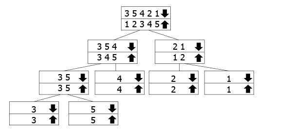
This tree is meant to represent how the recursive calls work. The arrays marked with the down arrow are the ones we call the function for, while we're merging the up arrow ones going back up. So you follow the down arrow to the bottom of the tree, and then go back up and merge.

In our example, we have the array 3 5 3 2 1, so we divide it into 3 5 4 and 2 1. To sort them, we further divide them into their components. Once we've reached the bottom, we start merging up and sorting them as we go.

If you'd like to read a detailed, dedicated article for Merge Sort, we've got you covered!

Implementation

The core function works pretty much as laid out in the explanation. We're just passing indexes left and right which are indexes of the left-most and right-most element of the subarray we want to sort. Initially, these should be 0 and array.length-1, depending on implementation.

The base of our recursion ensures we exit when we've finished, or when right and left meet each other. We find a midpoint mid, and sort subarrays left and right of it recursively, ultimately merging our solutions.

If you remember our tree graphic, you might wonder why don't we create two new smaller arrays and pass them on instead. This is because on really long arrays, this would cause huge memory consumption for something that's essentially unnecessary.

Merge Sort already doesn't work in-place because of the merge step, and this would only serve to worsen its memory efficiency. The logic of our tree of recursion otherwise stays the same, though, we just have to follow the indexes we're using:

public static void mergeSort(int[] array, int left, int right) {
                if (right <= left) return;
                int mid = (left+right)/2;
                mergeSort(array, left, mid);
                mergeSort(array, mid+1, right);
                merge(array, left, mid, right);
            }
            

To merge the sorted subarrays into one, we'll need to calculate the length of each and make temporary arrays to copy them into, so we could freely change our main array.

After copying, we go through the resulting array and assign it the current minimum. Because our subarrays are sorted, we just chose the lesser of the two elements that haven't been chosen so far, and move the iterator for that subarray forward:

 void merge(int[] array, int left, int mid, int right) {
                // calculating lengths
                int lengthLeft = mid - left + 1;
                int lengthRight = right - mid;
            
                // creating temporary subarrays
                int leftArray[] = new int [lengthLeft];
                int rightArray[] = new int [lengthRight];
            
                // copying our sorted subarrays into temporaries
                for (int i = 0; i < lengthLeft; i++)
                    leftArray[i] = array[left+i];
                for (int i = 0; i < lengthRight; i++)
                    rightArray[i] = array[mid+i+1];
            
                // iterators containing current index of temp subarrays
                int leftIndex = 0;
                int rightIndex = 0;
            
                // copying from leftArray and rightArray back into array
                for (int i = left; i < right + 1; i++) {
                    // if there are still uncopied elements in R and L, copy minimum of the two
                    if (leftIndex < lengthLeft && rightIndex < lengthRight) {
                        if (leftArray[leftIndex] < rightArray[rightIndex]) {
                            array[i] = leftArray[leftIndex];
                            leftIndex++;
                        }
                        else {
                            array[i] = rightArray[rightIndex];
                            rightIndex++;
                        }
                    }
                    // if all the elements have been copied from rightArray, copy the rest of leftArray
                    else if (leftIndex < lengthLeft) {
                        array[i] = leftArray[leftIndex];
                        leftIndex++;
                    }
                    // if all the elements have been copied from leftArray, copy the rest of rightArray
                    else if (rightIndex < lengthRight) {
                        array[i] = rightArray[rightIndex];
                        rightIndex++;
                    }
                }
            }
            

Time Complexity

If we want to derive the complexity of recursive algorithms, we're going to have to get a little bit mathy.

The Master Theorem is used to figure out time complexity of recursive algorithms. For non-recursive algorithms, we could usually write the precise time complexity as some sort of an equation, and then we use Big-O Notation to sort them into classes of similarly-behaving algorithms.

The problem with recursive algorithms is that that same equation would look something like this:

$$T(n) = aT(\frac{n}{b}) + cn^k$$

The equation itself is recursive! In this equation, a tells us how many times we call the recursion, and b tells us into how many parts our problem is divided. In this case that may seem like an unimportant distinction because they're equal for mergesort, but for some problems they may not be.

The rest of the equation is complexity of merging all of those solutions into one at the end. The Master Theorem solves this equation for us:

$$T(n) = \Bigg\{ \begin{matrix} O(n^{log_ba}), & a>b^k \\ O(n^klog n), & a = b^k \\ O(n^k), & a < b^k \end{matrix}$$

If T(n) is runtime of the algorithm when sorting an array of the length n, Merge Sort would run twice for arrays that are half the length of the original array.

So if we have a=2, b=2. The merge step takes O(n) memory, so k=1. This means the equation for Merge Sort would look as follows:

$$T(n) = 2T(\frac{n}{2})+cn$$

If we apply The Master Theorem, we'll see that our case is the one where a=b^k because we have 2=2^1. That means our complexity is O(nlog n). This is an extremely good time complexity for a sorting algorithm, since it has been proven that an array can't be sorted any faster than O(nlog n).

While the version we've showcased is memory-consuming, there are more complex versions of Merge Sort that take up only O(1) space.

In addition, the algorithm is extremely easy to parallelize, since recursive calls from one node can be run completely independently from separate branches. While we won't be getting into how and why, as it's beyond the scope of this article, it's worth to keep in mind the pros of using this particular algorithm.

Heapsort

Explanation

To properly understand why Heapsort works, you must first understand the structure it's based on - the heap. We'll be talking in terms of a binary heap specifically, but you can generalize most of this to other heap structures as well.

A heap is a tree that satisfies the heap property, which is that for each node, all of its children are in a given relation to it. Additionally, a heap must be almost complete. An almost complete binary tree of depth d has a subtree of depth d-1 with the same root that is complete, and in which each node with a left descendent has a complete left subtree. In other words, when adding a node, we always go for the leftmost position in the highest incomplete level.

If the heap is a max-heap, then all of the children are smaller than the parent, and if it's a min-heap all of them are larger.

In other words, as you move down the tree, you get to smaller and smaller numbers (min-heap) or greater and greater numbers (max-heap). Here's an example of a max-heap:

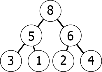
We can represent this max-heap in memory as an array in the following way:

8 5 6 3 1 2 4
            

You can envision it as reading from the graph level by level, left to right. What we have achieved by this is that if we take the kth element in the array, its children's positions are 2*k+1 and 2*k+2 (assuming the indexing starts at 0). You can check this for yourself.

Conversely, for the kth element the parent's position is always (k-1)/2.

Knowing this, you can easily "max-heapify" any given array. For each element, check if any of its children are smaller than it. If they are, swap one of them with the parent, and recursively repeat this step with the parent (because the new large element might still be bigger than its other child).

Leaves have no children, so they're trivially max-heaps of their own:

• 6 1 8 3 5 2 4: Both children are smaller than the parent, so everything stays the same.

• 6 1 8 3 5 2 4: Because 5 > 1, we swap them. We recursively heapify for 5 now.

• 6 5 8 3 1 2 4: Both of the children are smaller, so nothing happens.

• 6 5 8 3 1 2 4: Because 8 > 6, we swap them.

• 8 5 6 3 1 2 4: We got the heap pictured above!

Once we've learned to heapify an array the rest is pretty simple. We swap the root of the heap with the end of the array, and shorten the array by one.

We heapify the shortened array again, and repeat the process:

• 8 5 6 3 1 2 4

• 4 5 6 3 1 2 8: swapped

• 6 5 4 3 1 2 8: heapified

• 2 5 4 3 1 6 8: swapped

• 5 2 4 2 1 6 8: heapified

• 1 2 4 2 5 6 8: swapped

And so on, I'm sure you can see the pattern emerging.

Implementation

static void heapify(int[] array, int length, int i) {
                int leftChild = 2*i+1;
                int rightChild = 2*i+2;
                int largest = i;
            
                // if the left child is larger than parent
                if (leftChild < length && array[leftChild] > array[largest]) {
                    largest = leftChild;
                }
            
                // if the right child is larger than parent
                if (rightChild < length && array[rightChild] > array[largest]) {
                    largest = rightChild;
                }
            
                // if a swap needs to occur
                if (largest != i) {
                    int temp = array[i];
                    array[i] = array[largest];
                    array[largest] = temp;
                    heapify(array, length, largest);
                }
            }
            
            public static void heapSort(int[] array) {
                if (array.length == 0) return;
            
                // Building the heap
                int length = array.length;
                // we're going from the first non-leaf to the root
                for (int i = length / 2-1; i >= 0; i--)
                    heapify(array, length, i);
            
                for (int i = length-1; i >= 0; i--) {
                    int temp = array[0];
                    array[0] = array[i];
                    array[i] = temp;
            
                    heapify(array, i, 0);
                }
            }
            

Time Complexity

When we look at the heapify() function, everything seems to be done in O(1), but then there's that pesky recursive call.

How many times will that be called, in the worst case scenario? Well, worst-case, it will propagate all the way to the top of the heap. It will do that by jumping to the parent of each node, so around the position i/2. that means it will make at worst log n jumps before it reaches the top, so the complexity is O(log n).

Because heapSort() is clearly O(n) due to for-loops iterating through the entire array, this would make the total complexity of Heapsort O(nlog n).

Heapsort is an in-place sort, meaning it takes O(1) additional space, as opposed to Merge Sort, but it has some drawbacks as well, such as being difficult to parallelize.

Quicksort

Explanation

Quicksort is another Divide and Conquer algorithm. It picks one element of an array as the pivot and sorts all of the other elements around it, for example smaller elements to the left, and larger to the right.

This guarantees that the pivot is in its proper place after the process. Then the algorithm recursively does the same for the left and right portions of the array.

Implementation

static int partition(int[] array, int begin, int end) {
                int pivot = end;
            
                int counter = begin;
                for (int i = begin; i < end; i++) {
                    if (array[i] < array[pivot]) {
                        int temp = array[counter];
                        array[counter] = array[i];
                        array[i] = temp;
                        counter++;
                    }
                }
                int temp = array[pivot];
                array[pivot] = array[counter];
                array[counter] = temp;
            
                return counter;
            }
            
            public static void quickSort(int[] array, int begin, int end) {
                if (end <= begin) return;
                int pivot = partition(array, begin, end);
                quickSort(array, begin, pivot-1);
                quickSort(array, pivot+1, end);
            }
            

Time Complexity

The time complexity of Quicksort can be expressed with the following equation:

$$T(n) = T(k) + T(n-k-1) + O(n)$$

The worst case scenario is when the biggest or smallest element is always picked for pivot. The equation would then look like this:

$$T(n) = T(0) + T(n-1) + O(n) = T(n-1) + O(n)$$

This turns out to be O(n^2).

This may sound bad, as we have already learned multiple algorithms which run in O(nlog n) time as their worst case, but Quicksort is actually very widely used.

This is because it has a really good average runtime, also bounded by O(nlog n), and is very efficient for a large portion of possible inputs.

One of the reasons it is preferred to Merge Sort is that it doesn't take any extra space, all of the sorting is done in-place, and there's no expensive allocation and deallocation calls.

Performance Comparison

That all being said, it's often useful to run all of these algorithms on your machine a few times to get an idea of how they perform.

They'll perform differently with different collections that are being sorted of course, but even with that in mind, you should be able to notice some trends.

Let's run all of the implementations, one by one, each on a copy of a shuffled array of 10,000 integers:

time(ns)	Bubble Sort	Insertion Sort	Selection Sort	MergeSort	HeapSort	QuickSort
First Run	266,089,476	21,973,989	66,603,076	5,511,069	5,283,411	4,156,005
Second Run	323,692,591	29,138,068	80,963,267	8,075,023	6,420,768	7,060,203
Third Run	303,853,052	21,380,896	91,810,620	7,765,258	8,009,711	7,622,817
Fourth Run	410,171,593	30,995,411	96,545,412	6,560,722	5,837,317	2,358,377
Fifth Run	315,602,328	26,119,110	95,742,699	5,471,260	14,629,836	3,331,834
Sixth Run	286,841,514	26,789,954	90,266,152	9,898,465	4,671,969	4,401,080
Seventh Run	384,841,823	18,979,289	72,569,462	5,135,060	10,348,805	4,982,666
Eight Run	393,849,249	34,476,528	107,951,645	8,436,103	10,142,295	13,678,772
Ninth Run	306,140,830	57,831,705	138,244,799	5,154,343	5,654,133	4,663,260
Tenth Run	306,686,339	34,594,400	89,442,602	5,601,573	4,675,390	3,148,027

We can evidently see that Bubble Sort is the worst when it comes to performance. Avoid using it in production if you can't guarantee that it'll handle only small collections and it won't stall the application.

HeapSort and QuickSort are the best performance-wise. Although they're outputting similar results, QuickSort tends to be a bit better and more consistent - which checks out.

Sorting in Java

Comparable Interface

If you have your own types, it may get cumbersome implementing a separate sorting algorithm for each one. That's why Java provides an interface allowing you to use Collections.sort() on your own classes.

To do this, your class must implement the Comparable<T> interface, where T is your type, and override a method called .compareTo().

This method returns a negative integer if this is smaller than the argument element, 0 if they're equal, and a positive integer if this is greater.

In our example, we've made a class Student, and each student is identified by an id and a year they started their studies.

We want to sort them primarily by generations, but also secondarily by IDs:

public static class Student implements Comparable<Student> {
                int studentId;
                int studentGeneration;
            
                public Student(int studentId, int studentGeneration) {
                    this.studentId = studentId;
                    this.studentGeneration = studentGeneration;
                }
            
                @Override
                public String toString() {
                    return studentId + "/" + studentGeneration % 100;
                }
            
                @Override
                public int compareTo(Student student) {
                    int result = this.studentGeneration - student.studentGeneration;
                    if (result != 0)
                        return result;
                    else
                        return this.studentId - student.studentId;
                }
            }
            

And here's how to use it in an application:

public static void main(String[] args) {
                Student[] a = new SortingAlgorithms.Student[5];
                a[0] = new Student(75, 2016);
                a[1] = new Student(52, 2019);
                a[2] = new Student(57, 2016);
                a[3] = new Student(220, 2014);
                a[4] = new Student(16, 2018);
            
                Arrays.sort(a);
            
                System.out.println(Arrays.toString(a));
            }
            

Output:

[220/14, 57/16, 75/16, 16/18, 52/19]
            

Comparator Interface

We might want to sort our objects in an unorthodox way for a specific purpose, but we don't want to implement that as the default behavior of our class, or we might be sorting a collection of an built-in type in a non-default way.

For this, we can use the Comparator interface. For example, let's take our Student class, and sort only by ID:

public static class SortByID implements Comparator<Student> {
                public int compare(Student a, Student b) {
                    return a.studentId - b.studentId;
                }
            }
            

If we replace the sort call in main with the following:

Arrays.sort(a, new SortByID());
            

Output:

[16/18, 52/19, 57/16, 75/16, 220/14]
            

How it All Works

Collection.sort() works by calling the underlying Arrays.sort() method, while the sorting itself uses Insertion Sort for arrays shorter than 47, and Quicksort for the rest.

It's based on a specific two-pivot implementation of Quicksort which ensures it avoids most of the typical causes of degradation into quadratic performance, according to the JDK10 documentation.

Counting Sort

Counting Sort is a stable, non-comparative sorting algorithm, and it's main use is for sorting arrays of non-negative integers.

Counting Sort counts the number of objects that have distinct key values, and then applying a prefix sum on those counts to determine the position of each key in the output. Like all other non-comparative sorting algorithms, Counting Sort also performs the sort without any comparisons between the elements to be sorted. Also, being a stable sorting algorithm, Counting Sort preserves the order of the elements with equal keys sorted in the output array as they were in the original array.

This operation results in, essentially, a list of integer occurrences, which we typically name the count array. Counting Sort uses the auxilliary count array to determine the positions of elements:

Each index in the count array represents an element in the input array. The value associated with this index is the number of occurrences (the count) of the element in the input array.

The best way to get a feel of how Counting Sort works is by going through an example. Consider we have an array:

int[] arr = {0, 8, 4, 7, 9, 1, 1, 7};

For simplicity's sake, the elements in the array will only be single digits, that is numbers from 0 through 9. Since the largest value we can have is 9, let's label the maximum value as max = 9.

This is important because we'll need to designate a new count array, consisting of max + 1 elements. This array will be used for counting the number of occurrences of every digit within our original array we're given to sort, so we need to initialize the whole count array to 0, that is:

int[] countArray = {0, 0, 0, 0, 0, 0, 0, 0, 0, 0};

Since there are 10 possible elements our array can have, there are ten zero's for every single digit.

Since we've defined the array we'll be working on, and we have also defined our count array to keep count of each occurrence of a digit, we need to go through the following step to make Counting Sort work:

Step 1:

By going through our whole array arr in a single for loop, for every i from 0 to n-1, where n is the number of elements in arr, we'll count the occurrence of each digit by incrementing the value on the position arr[i] in our countArray. Let's see that in code:

for(int i = 0; i < arr.length; i++)
    countArray[arr[i]]++;

After the first step, our countArray looks like this: [1, 2, 0, 0, 1, 0, 0, 2, 1, 1].

Step 2:

Since we now have our countArray filled with values, we go on to the next step - applying prefix sums to the countArray. Prefix sums are basically formed when we add each of the previous numbers in the array onto the next accumulatively, forming a sum of all yet seen prefixes:

for(int i=1; i < countArray.length; i++)
    countArray[i] += countArray[i-1];

And after applying this step we get the following countArray: [1, 3, 3, 3, 4, 4, 4, 6, 7, 8].

Step 3:

The third and last step is calculating the element positions in the sorted output based off the values in the countArray. For this purpose, we'll need a new array that we'll call outputArray. The size of the outputArray is the same as our original arr, and we once again initialize this array to all zeros:

int[] outputArray = {0, 0, 0, 0, 0, 0, 0, 0};

As we've mentioned earlier, Counting Sort is a stable sort. If we iterated through our arr array from 0 to n-1 we may end up switching the elements around and ruin the stability of this sorting algorithm, so we iterate the array in the reverse order.

We'll find the index in our countArray that is equal to the value of the current element arr[i]. Then, at the position countArray[arr[i]] - 1 we'll place the element arr[i]. This guarantees we keep the stability of this sort. Afterwards, we decrement the value countArray[i] by one, and continue on doing the same until i >= 0:

for(int i = arr.length-1; i >= 0; i--){
    outputArray[countArray[arr[i]] - 1] = arr[i];
    countArray[arr[i]]--;
}

At the end of the algorithm, we can just copy the values from outputArr into our starting array arr and print the sorted array out:

for(int i = 0; i < arr.length; i++){
    arr[i] = outputArray[i];
    System.out.print(arr[i] + " ");
}

Running of course gives us the sorted array with guaranteed stability (relative order) of equal elements:

0 1 1 4 7 7 8 9

Complexity of Counting Sort

Let's discuss both the time and space complexity of Counting Sort.

Let's say that n is the number of elements in the arr array, and k is the range of allowed values for those n elements from 1...n. As we're working only with simple for loops, without any recursive calls, we can analyze the time complexity in a following manner:

• Counting the occurrence of each element in our input range takes O(n) time,
• Calculating the prefix sums takes up O(k) time,
• And calculating the outputArray based off the previous two takes O(n) time.

Accounting for all the complexities of these individual steps, the time complexity of Counting Sort is O(n+k), making Counting Sort's average case linear, which is better than most comparison based sorting algorithms. However, if the range of k is 1...n², the worst-case of Counting Sorts quickly deteriorates to O(n²) which is really bad.

Thankfully, this doesn't happen often, and there is a way to ensure that it never happens. This is how Radix Sort came to be - which typically uses Counting Sort as its main subroutine while sorting.

By employing Counting Sort on multiple bounded subarrays, the time complexity never deteriorates to O(n²). Additionally, Radix Sort may use any stable, non-comparative algorithm instead of Counting Sort, but it's the most commonly used one.

On the other hand, the space complexity problem is much easier. Since our countArray of size k is bigger than our starting array of n elements, the dominating complexity there will be O(k). Important thing to note is that, the larger the range of elements in the given array, larger is the space complexity of Counting Sort.

Radix Sort

Bucket Sort

The idea of bucket sort is quite simple, you distribute the elements of an array into a number of buckets and then sort those individual buckets by a different sorting algorithm or by recursively applying the bucket sorting algorithm.

You might have remembered, how shopkeepers or bank cashiers used to prepare/sort bundles of notes. They usually have a bucket load of cash with different denominations like 5, 10, 20, 50, or 100. They just put all 5 Rs notes into one place, all Rs 10 notes into another place, and so on.

This way all notes are sorted in O(n) time because you don't need to sort individual buckets, they are all same notes there.

Anyway, for bucket sort to work at its super fast speed, there are multiple prerequisites. First, the hash function that is used to partition the elements must be very good and must produce an ordered hash: if the i < j then hash(i) < hash(j).

If this is not the case then you cannot concatenate individual buckets in O(n) time. Second, the elements to be sorted must be uniformly distributed. If you still have trouble understanding Bucket sort or want to explore other linear time sorting algorithms,

Difference between Bucket Sort vs Counting Sort

If you keep these prerequisites aside, bucket sort is actually very good considering that counting sort is reasonably equal to its upper bound and counting sort is also super fast.

The particular distinction for bucket sort is that it uses a hash function to partition the keys of the input array, so that multiple keys may hash to the same bucket.  Hence each bucket must effectively be a growable list; similar to Radix sort, another O(n) sorting algorithm.
Many programmers get confused between Counting Sort and Bucket sort as they work quite similarly, but the most important difference between them is that Bucket sort uses a hash function to distribute keys while Counting sort creates a bucket for each key.

In our example, I have used JDK's Collections.sort() method to sort each bucket. This is to indicate that the bucket sort algorithm does not specify which sorting algorithm should be used to sort individual buckets.

A programmer may choose to recursively use bucket sort on each bucket until the input array is sorted, similar to radix sort. Anyway, whichever sorting method you use to sort individual buckets, the time complexity of bucket sort will still tend towards O(n).

I think there are perhaps greater similarities between the radix sort and bucket sort than there are between the counting sort and bucket sort.

Bucket Sort - FAQ

Now, let's see some of the frequently asked questions about Bucket sort in programming job interviews.

1. Is the bucket sort, a stable algorithm?
Bucket sort is not a stable sorting algorithm. If you remember,  A sorting algorithm is said to be stable if two objects with equal keys appear in the same order in sorted output as they appear in the input array to be sorted. Some sorting algorithms are stable by nature like Insertion sort, Merge Sort, or Bubble Sort, etc. In the case of Bucket sort, input sorts themselves by moving into a bucket and their order are not guaranteed to be retained.


2. Is the bucket sort in-place algorithm?
Bucket sort is also not an in-place sorting algorithm because you create buckets that can be array, linked list, or hashtable and they take additional spaces. In the worst of the good cases (sequential values, but no repetition) the additional space needed is as big as the original array.


3. What is the time complexity of Bucket sort?
The time complexity of bucket sort in the O(n) in the best and average case and O(n^2) in the worst case. The creation of bucket will take O(1) time and assume moving elements into the bucket will take O(1) time e.g. in the case of hashtable and linked list.

The main step is to sort elements on individual elements. This step also takes O(n) time on average if all numbers are uniformly distributed (please refer to CLRS book for more details). The last step to concatenate all buckets will also take O(n) time as there will be n items in all buckets

4. What is the time complexity of Bucket sort in the worst case?
The time complexity of bucket sort is O(n^2) in the worst case i.e. when all elements at allocated to the same bucket. Since individual buckets are sorted using another algorithm, if only a single bucket needs to be sorted, bucket sort will take on the complexity of the inner sorting algorithm. This is why bucket sort is only useful when the input is uniformly distributed in a range. This way they will not end up in the same bucket.


5. What is the space complexity of Bucket sort?
The space complexity of the bucket sort algorithm is O(n) because even in the worst of the good cases (sequential values, but no repetition) the additional space needed is as big as the original array. Please go through Algorithms and Data Structures - Part 1 and 2 courses on Pluralsight for more details on complexity analysis of various sorting algorithms in best, average, and worst case.

Java Program to implement Bucket Sort in Java

Problem Statement:
Given an unordered list of integers, rearrange them in the natural order.

Sample Input: {8,5,3,1,9,6,0,7,4,2,5}
Sample Output: {0,1,2,3,4,5,6,7,8,9,5}
Program to implement Bucket sort in Java

import java.util.ArrayList;
import java.util.Arrays;
import java.util.Collections;
import java.util.List;

/*
 * Java Program sort an integer array using radix sort algorithm.
 * input: [80, 50, 30, 10, 90, 60, 0, 70, 40, 20, 50]
 * output: [0, 10, 20, 30, 40, 50, 50, 60, 70, 80, 90]
 * 
 * Time Complexity of Solution:
 *     Best Case O(n); Average Case O(n); Worst Case O(n^2).
 * 
 */

public class BuckeSort {

  public static void main(String[] args) {

    System.out.println("Bucket sort in Java");
    int[] input = { 80, 50, 30, 10, 90, 60, 0, 70, 40, 20, 50 };

    System.out.println("integer array before sorting");
    System.out.println(Arrays.toString(input));

    // sorting array using radix Sort Algorithm
    bucketSort(input);

    System.out.println("integer array after sorting using bucket 
                         sort algorithm");
    System.out.println(Arrays.toString(input));

  }

  /**
   * 
   * @param input
   */
  public static void bucketSort(int[] input) {
    // get hash codes
    final int[] code = hash(input);
    
    // create and initialize buckets to ArrayList: O(n)
    List[] buckets = new List[code[1]];
    for (int i = 0; i < code[1]; i++) {
      buckets[i] = new ArrayList();
    }
    
    // distribute data into buckets: O(n)
    for (int i : input) {
      buckets[hash(i, code)].add(i);
    }
    
    // sort each bucket O(n)
    for (List bucket : buckets) {
      Collections.sort(bucket);
    }
    
    int ndx = 0;
    // merge the buckets: O(n)
    for (int b = 0; b < buckets.length; b++) {
      for (int v : buckets[b]) {
        input[ndx++] = v;
      }
    }
  }

  /**
   * 
   * @param input
   * @return an array containing hash of input
   */
  private static int[] hash(int[] input) {
    int m = input[0];
    for (int i = 1; i < input.length; i++) {
      if (m < input[i]) {
        m = input[i];
      }
    }
    return new int[] { m, (int) Math.sqrt(input.length) };
  }

  /**
   * 
   * @param i
   * @param code
   * @return
   */
  private static int hash(int i, int[] code) {
    return (int) ((double) i / code[0] * (code[1] - 1));
  }

}


Output
Bucket sort in Java
integer array before sorting
[80, 50, 30, 10, 90, 60, 0, 70, 40, 20, 50]
integer array after sorting using bucket sort algorithm
[0, 10, 20, 30, 40, 50, 50, 60, 70, 80, 90]

Bucket Sort - Important points to remember

Here are some important points about bucket sort you should remember, this is useful from both the interview and understanding point of view and the Interviewer expects that you know about them when you say that you know bucket sort.

1) Bucket Sort is also known as bin sort because you create bins or buckets to sort inputs.

2) Bucket sort is only useful when the input is uniformly distributed over a range like coins, numbers 1 to 100, etc.

3) You can use a linked list or array as a bucket. The choice of data structure will affect the insertion time e.g. if you use a linked list then adding on the head could take O(1) time. You can also use hash tables as buckets.

4) The bucket sort is one of the rare O(n) sorting algorithms i.e. time complexity of Bucket sort is the liner in the best and average case and not NLogN like Quicksort or Mergesort.

5) Bucket sort is not a stable sorting algorithm because in a stable algorithm if two input is same they retain their place in sorted order and in the bucket it depends upon how you sort the individual bucket. However, bucket sort can be made stable, known as radix sort, which we'll see in future articles.

6) You can sort the elements inside individual buckets either by recursively calling the bucket sort or using a separate sorting algorithm like insertion sort, bubble sort, or quicksort.

7) Is bucket sort an in-place sorting algorithm? No, it's not an in-place sorting algorithm. The whole idea is that input sorts themselves as they are moved to the buckets. In the worst of the good cases (sequential values, but no repetition) the additional space needed is as big as the original array.

8) The worst-case complexity of bucket sort, when all elements will end up in the same bucket is O(n^2) because then it has to be sorted by a different sorting algorithm.

9) The space complexity of bucket sort is O(n) because even to sort sequential values, without repetition, you need an array as big as the original array.


That's all about bucket sort in Java. It's one of the interesting sorting algorithms which gives you O(n) performance in the best and average case. Bucket sort should only be used when the input is uniformly distributed over a range e.g. numbers up to 1 to 1000.

You should also remember that Bucket sort is not a stable algorithm hence it's not guaranteed that equal keys on the input array will retain their places.

It is also not an in-place algorithm, as it will require additional space as big as the original array in the worst case. You can also refer following resources for more details on bucket sort and other O(n) sorting algorithms like Counting sort, Radix sort, etc.

Shell Sort

Most sorting algorithms compare elements, in our case numbers, which are near each other in some way. An example would be Bubble Sort, which compares adjacent elements and swaps them if needed. Shell Sort utilizes a completely different approach, comparing elements that are further apart in the beginning. Though, the further we sort, the closer they become.

The space between elements we are comparing (known as the gap) in the beginning can be given as one of the arguments when calling the algorithm. Shell Sort is considered to be a generalization of Insertion Sort, so it's useful to quickly draw a parallel between the two and recap Insertion Sort just in case.

Parallels with Insertion Sort

Insertion Sort places elements of a collection in their ordered place one at a time by selecting an element and comparing it with each element with a lower index. Once it finds the correct place for the current element, it's placed and the process repeats.

Here's a code snippet that should illustrate how Insertion Sort works. The whole collection is shifted to the right in the correct place to "free up" space for an element to be inserted.

public static void insertionSort(ArrayList<Integer> arr,int n) {
    int i, j, newValue;

    for (i = 1; i < n; i++) {
        newValue = arr.get(i);
        j = i;

        while (j > 0 && arr.get(j-1) > newValue) {
            arr.set(j,arr.get(j-1));
            j--;
        }
        arr.set(j,newValue);
    }
}

Shell Sort takes the insertion approach, but instead of assigning it its exact position, in each iteration it brings elements just closer to their place. Each pass will look a little more sorted, until it finally is.

To understand how this works, we must first explain what is a K-sorted array and what are its characteristics.

K-Sorted Array

Suppose A is an array of a size N. Array A is K-sorted if every element is, at most, K places away from its target position. In other words, for each i between 1 and N, the target place of A[i] is somewhere between i-K and 1+K in A.

For an unsorted, N-sized array, it is possible to K-sort it in O(N logK) time.

An important property of K-sorted arrays is that if K₁ sorted array is K₂-sorted, it stays K₁ sorted. This can easily be proven.

Case One

$$K_{1} > K_{2}$$

If A is K₁-sorted then every element from A is at most K₁ places away from its target position. If we then K₂-sort A then every element from A is at most K₂ places away from its target position. Since K₂ is smaller than K₁, if elements from A are at most K₂ places away from their target, then they must be closer than K₁ places from their target. That means that if A is K₂-sorted, it must be K₁-sorted.

Case Two

$$K_{1} < K_{2}$$

When A is K₁-sorted, if we K₂-sort it, no element will change place, because A already is K₂-sorted (explained in previous case). That means that it will also stay K₁-sorted.

Shell Sort Example

Unlike in Insertion Sort, where whenever we make a swap the collection is shifted to the right, in Shell Sort the elements whose positions we change get grouped together and then get sorted within the groups. After the groups are sorted, only then are they shifted, resulting is much less moving of the actual elements themselves.

A = [7, 13, 18, 22, 8, 29, 14, 7, 27, 25, 3]

Here, the number of elements is 11.

Now, we're supposed to choose a gap, between the elements we want to compare and then group:

$$gap = [\frac{11}{2}] = 5.$$

A: 7, 13, 18, 22, 8, 29, 14, 7, 27, 25, 3

Now, we make groups of numbers that are 5 elements apart (have 4 elements between them). The groups are (7, 29, 3), (13, 14), (18, 7), (22, 27), (8, 25).

Since N/2 is used for the initial gap value, the first group has 3 elements, and others have two elements each due to the fact our collection has an uneven number of elements.

A: 7, 13, 18, 22, 8, 29, 14, 7, 27, 25, 3

There are no elements in the first group with smaller index than 0, so we are starting from second index - whose value is 29. The next step is to compare 29 to all the elements in the group with smaller indexes.

• 7 < 29 is true so their places will not be swapped.

There are no other elements in the group with an index lower than 5, so we are finished with A[5].

The next number in the group is 3, whose original index is 10:

• 29 < 3 is false so they will be swapped:

A: 7, 13, 18, 22, 8, 3, 14, 7, 27, 25, 29

Now, the value of A[5] is 3. 29 must be on its ordered place in the group, because there is no element with greater index in that group. 3, on the other hand, might still be smaller than group members with lower indexes.

• 7 < 3 is false, so they will be swapped:

A: 3, 13, 18, 22, 8, 7, 14, 7, 27, 25, 29

There are no elements in A with a lower index than 10 that we haven't already compared to A[10]. All the members of the first group are now sorted.

The next group is (13, 14):

A: 3, 13, 18, 22, 8, 7, 14, 7, 27, 25, 29

It is easy to notice that if there are only two elements in the group, they are swapped only if the first one is bigger that the second one. The groups that are left now are (18, 7), (22, 27), and (8, 25) and the only group that will need swapping will be (18, 7):

A: 3, 13, 7, 22, 8, 7, 14, 18, 27, 25, 29

At this point there are no groups left to analyze, so the array is 5-sorted. Although looking better than before, it's still not quite finished.

Now, the gap is divided by two yet again:

$$gap = [\frac{5}{2}] = 2$$

Now, we make groups of elements that are just 2 elements apart, which means that there is only one element between them. These groups are (3, 7, 8, 14, 27, 29) and (13, 22, 7, 18, 25):

A: 3, 13, 7, 22, 8, 7, 14, 18, 27, 25, 29

Sorting when gap is 2 will be displayed on the 2-sorting of the second group.

A: 3, 13, 7, 22, 8, 7, 14, 18, 27, 25, 29

These two groups are sorted in the same way the previous groups were sorted, and we're left with:

A: 3, 7, 7, 13, 8, 18, 14, 22, 27, 25, 29

The last thing left to do is to 1-sort the array, which is, actually Insertion Sort.

Every member is compared to all other elements with smaller indexes. The important thing to notice here is that array is already 2-sorted, so it is only possible that elements on places i and i+1 are not ordered. Therefore, when 1-sorting, only elements next to each other can be swapped.

Implementation

With all of the above in mind, let's implement Shell Sort. The loop invariant in the main for loop is that the array is gap-sorted. The gap is halved on every iteration until it reaches 0. When it does, the array is sorted:

public static void shSort(ArrayList<Integer> arr,int n) {
    for (int gap = n/2; gap > 0; gap /= 2) {
        for (int i = gap; i < n; i+= 1) {

            int temp = arr.get(i);
            int j;
            for (j = i; j >= gap && arr.get(j-gap) > temp; j -= gap)
                arr.set(j,arr.get(j-gap));
            arr.set(j,temp);
        }
    }
}

The array and its size are given as arguments of the method and the loop gets executed log_n times.

The first nested for loop goes through groups of elements that are gap places apart. That loop gets executed n-gap times. The temp variable is necessary for swapping, as usual.

One of the conditions in the second nested for loop is that j > gap, because we are comparing an element to all members of the group with smaller indexes from right to left.

Due to this, the last number that will be observed will be the first member of the group. The second condition is that j-gap < temp. This means that the loop is being executed while there are elements with lower indexes that are bigger than arr[j].

The first one that is lower breaks the loop. Then, arr[j] gets moved to the index whose value it was smaller than. This loop repeats i/gap times.

Time Complexity

Let us now calculate the time complexity of Shell Sort. As was already mentioned, the first loop is executed log_n times.

The second loop starts with gap as the index, which is 2^k. Since in the third loop we subtract gap, that means that in the sum, i should be divided by gap:

*Scroll to view*

This all brings the time complexity to O(n logn). Here, we assumed the fact that gap is set to n/2.

Conclusion

Shell Sort compares elements that are further apart in the beginning, though, the further we sort, the closer they become resulting in an array that's a bit more sorted after each iteration.

Shell Sort performs better than Insertion Sort but it has a bigger cache miss ratio than Quick Sort.

Conclusion

Sorting is a very common operation with datasets, whether it is to analyze them further, speed up search by using more efficient algorithms that rely on the data being sorted, filter data, etc.

Sorting is supported by many languages and the interfaces often obscure what's actually happening to the programmer. While this abstraction is welcome and necessary for effective work, it can sometimes be deadly for efficiency, and it's good to know how to implement various algorithms and be familiar with their pros and cons, as well as how to easily access built-in implementations.